SAND TANKS
SOUTHERN MARICOPA COUNTY, ARIZONA
![]()
INTRODUCTION
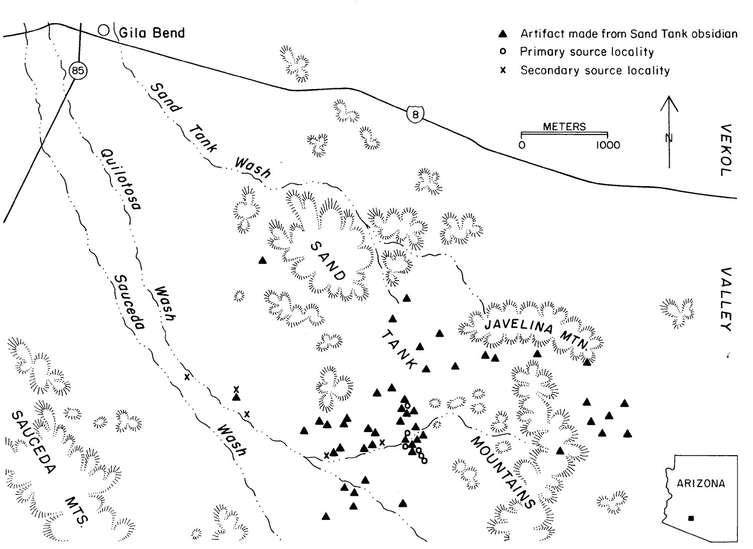
In January 1998 this laboratory and SWCA Inc., undertook a field mapping and collection survey of a previously unreported source of archaeological obsidian on the Barry M. Goldwater Range in far southwestern Maricopa County, Arizona. The survey included an intensive field examination and recording of the primary in-situ marekanites (obsidian nodules) in the western Sand Tank Mountains as well as an examination of the secondary distribution through Quilotosa Wash system that ultimately drains into the Gila River. There appears to be little chemical variability within the incompatible element composition of the source, and the secondary distribution is only apparent little more than 15 kilometers downstream. Possibly due to the source location away from major prehistoric trail systems and its rather limited secondary distribution, Sand Tanks obsidian does not seem to have been a major raw material source in prehistory, despite nodule sizes up to 65 mm in diameter and quite high density at the primary sources (Shackley 1995; Tucker 1996). It apparently was not as "popular" a raw material in prehistory compared to Sauceda Mountains which is located only a few tens of kilometers to the south, but likely along frequented trail systems; systems probably predicated on the location of the Sauceda Mountains source.
The geology of the Sand Tanks source seems rather typical of rhyolite dome systems of Tertiary volcanic arcs. The remnant marekanites are present within eroding obsidian zones on domes primarily comprised of perlite and vitrophyre, with some crystalline lava.
SILICIC GEOLOGY AND SECONDARY DEPOSITION
Introduction
There has been virtually no intensive geological investigation of the silicic geology in this part of Maricopa County (see Reynolds et al. 1986; Scarborough 1986; and Wilson et al. 1957). Wilson et al.’s (1957) general county map, while not defining the complexity evident in the field, notes an area on the eastern flank of the Sand Tank mountains as "Sauceda Volcanics (Ksv) Cretaceous in age including rhyolite, latite, and andesite. Locally contains volcanic glass." This, of course, also includes another glass source named the Sauceda Mountains or South Sauceda Mountains (Shackley 1988, 1990, 1995). Whether Wilson and the others actually located obsidian in the field at Sand Tanks will never be known, but based on the field geology, it certainly seems reasonable that Sauceda and Sand Tanks are contemporaneous. The geochemistry, however, does not suggest common magmatic origin despite proximity (see Hughes and Smith 1993; Shackley 1995, 1998a, 1998b).
Field Relations and Obsidian Deposition
Following will be a brief synopsis of the field relations as observed in the field, descriptions of the character of the rhyolite domes that produced the glass at Sand Tanks including density of marekenites and prehistoric reduction debris, the secondary distribution of the source, and some comments on the elemental composition of the source.
The primary Sand Tanks obsidian source is located on the western margin of the Sand Tanks Mountains in the west central area of the Kaka NW, Arizona, Provisional 7.5’ Quad, 1986 in Maricopa County, Arizona. Generally, the Sand Tanks appear to be part of the bimodal or trimodal Sauceda Volcanics with a basal Tertiary series of rhyolitic eruptive events, followed by intermediate and finally Quaternary mafic eruptions. The basement rock appears to be dominated by younger Precambrian granites with some older metamorphics. The production of rhyolite in the Tertiary may be due to crustal remelting of the silicic basement particularly the granites.
While extremely eroded at this time, the dome structures appear to be a series of coalesced events oriented from northwest (UTM 12 N3618043 E360508 ± 1m) to southeast (UTM 12 N3616703 E361307 corrected). Exposures of rhyolite lava frequently consist of perlitic and vitrophyric glass with marekenites up to 60 mm in diameter that appear to be remnants within the devitrified lava, particularly evident at Localities 1a, b, and c (Sample numbers 111197-1), but also evident at Localities 2-4. This is a typical pattern in Sonoran Desert Tertiary glass sources (Shackley 1998, 1990, 1995). Parenthetically, primary embedded marekenites have never been discovered for the Sauceda Mountains source, despite a much higher density of nodules in the alluvium and greater popularity as a raw material prehistorically. It is possible that the original glassy obsidian zones on the domes at Sauceda have been completely eroded away or this type of environment simply hasn’t been located.
Sampling Strategy and Locality Descriptions
The primary coalesced domes were stratified into four collection localities based mainly on a decrease in the density of marekenites evident on the surface between the localities and the presence remnant artifact quality marekanites within perlitic lava. They are all certainly part of one geological event, however. At Localities 1a and 3, surface collection units were placed in the perceived densest areas to generate density estimates. Samples were also collected and bagged at each locality for chemical analysis (Figure 1).
Locality 1A (UTM N3617714 E360501 ± 1m; sample numbers 111197-1-). This is a large (» 200m diameter) eroded dome with ashy perlitic lava. On the west side of the dome small eroded areas of perlitic lava occur with embedded marekanites. Typical of most of these localities, it appears that the marekenites were pyroclasts within an ashy eruption. The lava has devitrified over time while the marekenites are vitric remnants within the flow (see Bouška 1993:99; Figure 2 here). The maximum size nodule located was 64.5 mm in diameter. One 2 X 2m collection unit (UTM N3617718 E360503 ± 1m) yielded 110 nodules from 3.8mm to 42 mm in diameter, probably a relatively representative sample of the most dense portion of the site. Two bipolar core fragments and two bipolar/interior flakes were recovered in this collection unit. This ratio (100 geological samples to four artifacts) is the general density of nodules to artifacts at the source.
Locality 1B. This locality is at the northern base of Locality 1A dome and is comprised of a large perlitic lava exposure with a lower marekanite density (» 2-3 /5cm2). The exposure is mainly due to erosion by an ephemeral wash at the base of the dome. No artifacts were located at this locality.
Locality 1C (UTM 12 N3617834 E360561 ± 1m). This is a small exposure of perlitic lava with marekanites in between Localities 1 and 2, and cannot be related either structure. The largest nodule located was 40.8mm in diameter.
Locality 2 (UTM 12 N3618043 E360508 ± 1m; sample numbers 111197-2-). This is a dome structure immediately north of Locality 1 and mainly consists of a large exposure 50+ m in length along the southern margin of the dome on the edge of upper Quilotosa Wash. The density of the marekenites in the perlitic matrix is up to 73/50cm2, most smaller than 30 mm in diameter. Some of the nodules appear to have been reduced possibly to remove them from the matrix (Figure 3) . The largest nodule located was 40.8mm in diameter.
Locality 3 (UTM 12 N3616984 E361205 corrected; sample numbers 111297-1-). A smaller dome structure (50-75 m in diameter) than the others, Locality 3 is located about 1 km southeast of Locality 1. There is no evidence of in-situ marekanites here, but the density of nodules in the regolith is relatively high (Figure 4). A 3 X 3m surface collection unit yielded 101 nodules from seven to 32.5mm in diameter and one bipolar flake. The largest nodule was 55.6mm in diameter. The lack of in-situ nodules and perlitic lava here is probably the result of either alluviation and colluviation covering the basement rock and/or a more ashy eruptive phase where the marekanites remaining were pyroclasts in a gaseous eruption sequence. Here and at Locality 4 (UTM 12 N3616703 E361307 corrected; sample numbers 111292-2-), rather than dome remnants, they may actually be secondary deposits probably emplaced during the eruptive events from the domes at Localities 1 and 2.
Secondary Deposition
The recognition of secondary depositional effects in the prehistoric procurement of obsidian in the Southwest has recently become an important issue (Shackley 1992, 1998a; see Shelley 1993). Sauceda Mountains obsidian appears to erode from the South Sauceda Mountains to the Gila River to the north (Shackley 1988, 1990). A primary goal of the Sand Tanks obsidian project was to determine the extent of the secondary distribution of the source and determine whether it mixed with the Sauceda nodules in the Sauceda Wash. Survey of the Quilotosa Wash system from Locality 1 to Sauceda Wash did indicate some secondary erosion of the nodules, but only for about 15 km downstream. This indicates that 1) the density of nodules at Sand Tanks is not as great as Sauceda Mountains material, and 2) the Sand Tanks and Sauceda source material does not mix into the Sauceda Wash, and therefore 3) the Sand Tanks obsidian does not make it to the Gila River.
Pea size nodules are all that are left by the time the Black Butte area is reached along the Quilotosa Wash, considerably braided at this point and beginning to blend with Sauceda Wash. The last collection point (111297-7) around UTM 12 N3622199 E345668 corrected (USGS Hat Mountain 7.5’ Quad 1986), yielded only 3 small pea-sized nodules in 20-30 minutes survey. Four other collection localities in the wash system upstream yielded increasing size and quantity of nodules (surveyed all for 20-30 minutes; see Table 2 for the elemental characterization of these specimens).
LABORATORY SAMPLING, ANALYSIS AND INSTRUMENTATION
Forty-three source standards from primary geological contexts and secondary deposits were analyzed by EDXRF (see below). Nodules were selected using a stratified random sampling strategy, stratified based on locality and nodule size over 10 mm in diameter (Davis et al. 1998). After brush-washing, selected nodules over 15 mm in diameter were hammer-split to expose a fresh surface for analysis. Nodules between 10 and 15 mm in diameter were not split, but analyzed whole.
The results presented here are quantitative in that they are derived from "filtered" intensity values ratioed to the appropriate x-ray continuum regions through a least squares fitting formula rather than plotting the proportions of the net intensities in a ternary system (McCarthy and Schamber 1981; Schamber 1977). Or more essentially, these data through the analysis of international rock standards, allow for inter-instrument comparison with a predictable degree of certainty (Hampel 1984).
The trace element analyses were performed in the Department of Geology and Geophysics, University of California, Berkeley, using a SpectraceÔ 400 (United Scientific Corporation) energy dispersive x-ray fluorescence spectrometer. The spectrometer is equipped with a Rh x-ray tube, a 50 kV x-ray generator, with a Tracor X-ray (SpectraceÔ ) TX 6100 x-ray analyzer using an IBM PC based microprocessor and Tracor reduction software. The x-ray tube was operated at 30 kV, 0.20 mA, using a 0.127 mm Rh primary beam filter in a vacuum path at 250 seconds livetime to generate x-ray intensity Ka -line data for elements titanium (Ti), manganese (Mn), iron (as FeT), zinc (Zn), thorium (Th), rubidium (Rb), strontium (Sr), yttrium (Y), zirconium (Zr), and niobium (Nb). Weight percent iron (Fe2O3T) can be derived by multiplying ppm estimates by 1.429710-4. X-ray intensity Ka -line data for barium (Ba), lanthanum (La), and cerium (Ce) were determined by using a 241Am gamma ray source for 500 seconds livetime in an air path (see Davis et al. 1998). Trace element intensities were converted to concentration estimates by employing a least-squares calibration line established for each element from the analysis of international rock standards certified by the National Institute of Standards and Technology (NIST), the US. Geological Survey (USGS), Canadian Centre for Mineral and Energy Technology, and the Centre de Recherches Pétrographiques et Géochimiques in France (Govindaraju 1994). Further details concerning the petrological choice of these elements in Southwest obsidians is available in Shackley (1988, 1990, 1992, 1995; also Mahood and Stimac 1991; and Hughes and Smith 1993). Specific standards used for the best fit regression calibration for elements Ti through Nb include G-2 (basalt), AGV-1 (andesite), GSP-1 and SY-2 (syenite), BHVO-1 (hawaiite), STM-1 (syenite), QLM-1 (quartz latite), RGM-1 (obsidian), W-2 (diabase), BIR-1 (basalt), SDC-1 (mica schist), TLM-1 (tonalite), SCO-1 (shale), all US Geological Survey standards, and BR-N (basalt) from the Centre de Recherches Pétrographiques et Géochimiques in France (Govindaraju 1994). In addition to the reported values here Ni, Cu, Zn, Th, La, Ce, Pr, Nd, and Sm were measured, but these are not consistently useful in discriminating glass sources and are not generally reported. These data are available on disk by request.
The approximate practical detection limits of the elements of interest that include error imposed by inter-element interference are as follows: Ti 23 ppm; Mn 40 ppm; Fe 10 ppm; Pb 8 ppm; Rb 5 ppm; Sr 3.5 ppm; Y 7 ppm; Zr 7 ppm; Nb 8 ppm; Ba 20 ppm; La 20 ppm; Ce 20 ppm. These are the smallest amounts that can be quantitatively measured, defined as a signal which is six standard deviation units above background (6S ).
The data from the Tracor software were translated directly into Excel™ for Windows software for manipulation and on into SPSS™ for Windows for statistical analyses. In order to evaluate these quantitative determinations, machine data were compared to measurements of known standards during each run. Table 1 shows a comparison between values recommended for three international obsidian and rhyolite rock standards, RGM-1, NBS(SRM)-278, and JR-2. One of these standards is analyzed during each sample run to check machine calibration. The results shown in Table 1 indicate that the machine accuracy is quite high, particularly for the mid-Z elements, and other instruments with comparable precision should yield comparable results. Further information on the laboratory instrumentation can be found in Shackley (1995) and on the lab analysis page.
Trace element data exhibited in Tables 1 and 2 are reported in parts per million (ppm), a quantitative measure by weight.
Data Interpretation
Data and data reduction for the elemental analysis are displayed in Tables 1 and 2 and graphs below. The central tendency data in Table 3 and the plots indicate a real lack of elemental variability unlike the Sauceda Mountains material (Shackley 1995). Figure 7 includes the some of the small nodule secondary source deposit material, and the variability noted here is a result of small mass and its effect on the elemental analysis by EDXRF not inherent source variability (see Davis et al. 1998). This lack of elemental variability and the small number of primary eruptive centers suggests that the obsidian producing rhyolite was produced over a very short period of time and/or limited fractionation occurred in the magma chamber (Hildreth 1981; Mahood & Stimac 1990; Shackley 1998b). This is very unlike the Sauceda Mountains case where there is a bimodal character to the incompatible element composition that may be spatially oriented and suggests a longer eruptive history (Shackley 1995).
SUMMARY AND CONCLUSIONS
The Sand Tanks obsidian source appears to be one of the most unique sources in the Southwest. The marekanites available are of equal quality and nodule size of any of the Tertiary period sources in western North America, and yet the source was not exploited by prehistoric knappers to any real extent (see Tucker 1996). Of 220 samples analyzed from Classic Period contexts at Pueblo Grande in the Phoenix Basin, only four (.02%) exhibit the elemental concentrations consistent with Sand Tanks (originally assigned as an unknown), while Sauceda Mountains contributed 67 (30%; see Peterson et al. 1997). Perhaps more importantly, an analysis of 75 obsidian artifacts from Sedentary period contexts at the Gatlin Site near Gila Bend yielded 64 artifacts (85.3%) from Sauceda Mountains and none from Sand Tanks; the rest were from Unknown A, Vulture, Superior, and Los Vidrios (Doyel 1996; Shackley 1995). If any of the Los Vidrios material were procured directly by the Gatlin Site inhabitants, then travel would have to come close at least to the secondary deposits of Sand Tanks. So, it appears that north-south communication during the Sedentary Period and east-west travel during the Classic Period in some way circumvented the Sand Tanks source. The near lack of any reduced nodules at Sand Tanks is also indicative of a lack of interest in the source during prehistory.
An examination of the files at the Berkeley lab indicates that Pueblo Grande is the only site any distance from southern Maricopa County where this source has occurred. All four specimens at Pueblo Grande from the Sand Tanks source were unreduced marekanites that could have been carried into the site along with Sauceda material procured as secondary deposits in the Black Butte area. We will never know.
What is important here is that the paucity of Sand Tanks obsidian in prehistoric contexts outside the immediate area certainly suggests that Sauceda Mountains continued to be part of a procurement/interaction sphere throughout prehistory, probably for changing rationale, and that Sand Tanks was located in an area where fewer prehistoric groups visited for long enough to procure obsidian. The primary reason, however, is probably that Sauceda Mountains obsidian occurs over a wide geographic area in relatively high density and was evidently on a major north-south and east-west communication route or at least became a regular part of exchange relations in those directions.
The Sand Tanks obsidian source remains one of the most unique sources of archaeological obsidian in the world, simply because it was ignored in prehistory.
![]()
Table 1. Elemental concentrations for Sand Tanks primary localities (111197-) and secondary deposits (111297-)
| SAMPLE | Ti |
Mn |
Fe |
Zn |
Th |
Rb |
Sr |
Y |
Zr |
Nb |
Ba |
La |
Ce |
111197-1-9 |
1067.6 |
595.4 |
11101.2 |
52.6 |
22.8 |
170.0 |
4.7 |
36.1 |
263.6 |
29.0 |
46.8 |
38.7 |
95.2 |
8 |
1126.7 |
606.1 |
11306.8 |
58.1 |
24.9 |
173.9 |
9.2 |
41.4 |
268.3 |
31.9 |
|||
4 |
1048.8 |
570.7 |
11335.1 |
55.8 |
26.4 |
173.5 |
8.9 |
37.5 |
267.2 |
30.8 |
59.2 |
42.7 |
99.0 |
5 |
1251.2 |
600.6 |
11879.6 |
65.0 |
20.2 |
177.2 |
6.3 |
41.4 |
268.1 |
33.0 |
56.2 |
45.4 |
104.0 |
10 |
1087.2 |
551.1 |
10792.8 |
55.1 |
16.3 |
164.7 |
8.1 |
43.7 |
258.6 |
29.4 |
49.2 |
39.7 |
84.8 |
3 |
1136.5 |
691.2 |
12414.7 |
60.0 |
25.6 |
178.2 |
7.2 |
38.6 |
270.4 |
33.7 |
51.4 |
38.6 |
96.2 |
6 |
1242.1 |
532.1 |
11308.1 |
53.7 |
23.5 |
170.8 |
8.7 |
34.1 |
264.8 |
31.9 |
54.4 |
44.5 |
98.7 |
1 |
1227.0 |
612.9 |
11534.7 |
61.5 |
29.9 |
176.1 |
7.9 |
37.3 |
262.8 |
29.1 |
52.8 |
44.4 |
103.1 |
11 |
1196.8 |
621.0 |
11886.6 |
60.4 |
30.8 |
182.6 |
8.8 |
36.6 |
274.0 |
30.9 |
53.5 |
44.4 |
101.6 |
7 |
956.0 |
540.0 |
10895.9 |
53.0 |
27.9 |
164.4 |
8.7 |
39.9 |
256.8 |
33.6 |
54.4 |
44.8 |
110.4 |
2 |
1155.0 |
621.1 |
11202.2 |
56.3 |
23.5 |
167.8 |
8.1 |
41.3 |
259.2 |
30.8 |
45.4 |
31.4 |
86.1 |
LOCUS 1C -1 |
1001.1 |
547.8 |
11092.7 |
59.6 |
21.7 |
167.2 |
7.4 |
39.6 |
254.9 |
31.5 |
45.3 |
43.0 |
102.5 |
2 |
1019.2 |
518.1 |
10789.7 |
58.9 |
16.4 |
163.9 |
6.3 |
37.0 |
248.3 |
29.5 |
40.0 |
43.5 |
98.4 |
3 |
981.9 |
483.0 |
10389.7 |
55.8 |
26.6 |
159.4 |
6.8 |
40.0 |
248.0 |
26.0 |
39.3 |
36.1 |
80.9 |
111197-2-5 |
985.6 |
557.9 |
10505.4 |
51.2 |
22.8 |
161.2 |
5.5 |
40.5 |
248.3 |
28.2 |
43.8 |
40.0 |
94.1 |
4 |
1575.2 |
742.2 |
13502.1 |
62.3 |
34.2 |
180.4 |
9.1 |
38.6 |
260.8 |
30.8 |
48.5 |
40.4 |
95.1 |
2 |
1052.4 |
523.0 |
10586.1 |
53.1 |
23.4 |
164.5 |
5.5 |
38.2 |
254.0 |
29.8 |
46.4 |
39.4 |
89.7 |
3 |
1103.5 |
589.0 |
11792.6 |
59.3 |
26.3 |
175.4 |
9.7 |
41.0 |
257.1 |
34.0 |
41.7 |
42.4 |
105.8 |
1 |
1143.5 |
577.6 |
11027.0 |
56.6 |
29.2 |
171.6 |
6.0 |
37.7 |
253.5 |
36.7 |
43.6 |
47.3 |
98.7 |
111197-4-1 |
1113.7 |
641.5 |
12212.3 |
56.9 |
25.3 |
186.1 |
7.7 |
37.6 |
270.2 |
32.9 |
56.7 |
46.5 |
101.6 |
3 |
1171.5 |
601.6 |
11668.9 |
58.8 |
26.4 |
176.2 |
8.4 |
40.7 |
266.3 |
33.9 |
43.7 |
45.7 |
93.8 |
4 |
1170.5 |
575.0 |
11430.5 |
55.7 |
22.7 |
169.6 |
5.8 |
34.1 |
263.8 |
33.8 |
54.7 |
44.9 |
102.2 |
6 |
974.1 |
651.1 |
12047.8 |
64.1 |
23.6 |
178.0 |
9.1 |
40.7 |
268.4 |
32.3 |
|||
2 |
1197.0 |
616.5 |
11703.4 |
58.4 |
20.3 |
170.3 |
9.2 |
38.8 |
267.2 |
33.0 |
|||
1 |
931.2 |
497.4 |
10463.4 |
46.7 |
21.9 |
153.5 |
7.9 |
36.7 |
254.2 |
28.2 |
|||
111197-3-7 |
1205.6 |
554.7 |
11184.0 |
49.7 |
24.3 |
168.5 |
4.7 |
33.6 |
253.9 |
28.7 |
48.6 |
45.2 |
101.6 |
1 |
1069.5 |
591.8 |
11631.7 |
57.3 |
26.7 |
171.0 |
8.5 |
35.1 |
269.8 |
31.6 |
|||
6 |
1181.2 |
585.4 |
11416.3 |
55.8 |
28.4 |
172.0 |
10.8 |
36.3 |
264.9 |
30.1 |
51.7 |
50.5 |
101.8 |
4 |
1201.5 |
623.9 |
11851.9 |
56.7 |
30.2 |
180.9 |
8.2 |
39.7 |
276.4 |
30.5 |
42.4 |
42.2 |
83.1 |
5 |
1026.5 |
651.0 |
11383.6 |
56.0 |
31.9 |
175.2 |
8.3 |
40.0 |
268.8 |
30.6 |
47.2 |
46.2 |
94.7 |
3 |
1135.1 |
592.7 |
11399.4 |
51.8 |
26.2 |
177.2 |
8.0 |
39.7 |
268.5 |
32.7 |
54.8 |
54.3 |
106.8 |
2 |
1210.5 |
578.5 |
11686.7 |
52.7 |
21.4 |
163.8 |
6.9 |
36.8 |
256.5 |
27.5 |
44.8 |
46.9 |
97.8 |
111297-3-3 |
1063.6 |
572.8 |
11097.4 |
53.5 |
29.3 |
165.1 |
7.6 |
37.4 |
252.7 |
32.2 |
|||
1 |
1192.0 |
715.5 |
12897.9 |
63.0 |
28.4 |
171.5 |
8.7 |
36.4 |
257.1 |
27.7 |
|||
2 |
1069.3 |
514.9 |
10977.8 |
56.5 |
27.2 |
166.6 |
5.6 |
36.8 |
263.0 |
33.0 |
|||
111297-5-2 |
1066.6 |
509.0 |
10859.2 |
51.3 |
18.5 |
158.4 |
8.0 |
37.3 |
254.3 |
31.2 |
|||
1 |
1142.5 |
556.0 |
11117.9 |
54.8 |
28.3 |
157.8 |
5.6 |
29.5 |
242.0 |
28.2 |
|||
111297-6-1 |
912.3 |
331.7 |
8809.9 |
44.0 |
0.0 |
101.9 |
15.9 |
25.1 |
180.7 |
20.6 |
|||
2 |
1242.3 |
526.4 |
11641.7 |
55.0 |
22.0 |
160.0 |
7.1 |
33.4 |
243.3 |
26.7 |
|||
3 |
1180.7 |
572.9 |
11363.3 |
55.1 |
27.6 |
167.1 |
8.7 |
38.0 |
254.0 |
27.3 |
|||
11112-7-3 |
1028.2 |
447.5 |
10177.3 |
54.3 |
15.5 |
135.5 |
7.5 |
32.9 |
211.0 |
28.2 |
|||
2 |
898.4 |
295.7 |
8549.1 |
41.3 |
0.0 |
111.1 |
7.0 |
27.8 |
177.8 |
27.6 |
|||
1 |
1072.2 |
357.8 |
8511.2 |
37.1 |
22.2 |
113.9 |
4.3 |
22.9 |
175.0 |
19.6 |
Table 2. Mean and central tendency for elemental concentrations from the Sand Tanks primary localities (from data in Table 1).
| Element | ||||||
|---|---|---|---|---|---|---|
N |
Minimum |
Maximum |
Mean | Std. Error of Mean |
1 S.D. |
|
| Ti | 32 | 931.2 | 1575.2 | 1123.291 | 21.673 | 122.599 |
| Mn | 32 | 483.0 | 742.2 | 588.811 | 9.544 | 53.987 |
| Fe | 32 | 10389.7 | 13502.1 | 11419.472 | 112.015 | 633.653 |
| Zn | 32 | 46.7 | 65.0 | 56.528 | .717 | 4.055 |
| Th | 32 | 16.3 | 34.2 | 25.056 | .726 | 4.105 |
| Rb | 32 | 153.5 | 186.1 | 171.409 | 1.281 | 7.245 |
| Sr | 32 | 4.7 | 10.8 | 7.706 | .262 | 1.480 |
| Y | 32 | 33.6 | 43.7 | 38.432 | .427 | 2.418 |
| Zr | 32 | 248.0 | 276.4 | 262.110 | 1.362 | 7.703 |
| Nb | 32 | 26.0 | 36.7 | 31.131 | .405 | 2.289 |
| Ba | 27 | 39.3 | 59.2 | 48.754 | 1.069 | 5.553 |
| La | 27 | 31.4 | 54.3 | 43.305 | .868 | 4.508 |
| Ce | 27 | 80.9 | 110.4 | 97.312 | 1.408 | 7.314 |
To matrix, biplots, and 3-D plots of the data
To matrix, biplots, and 3-D plots of the data
To matrix, biplots, and 3-D plots of the data ![]()
![]()
This page maintained by Steve Shackley (shackley@berkeley.edu).
Copyright © 2001 M. Steven Shackley. All rights reserved.
Revised: Saturday, 21 March 2015 04:53:16 AM -0800